A Guide to Zero-Day Attack Detection with Denoising Autoencoders

Zero-day attacks are among the most serious cybersecurity threats. They exploit previously unknown vulnerabilities, allowing them to bypass existing intrusion detection systems (IDS). Traditional signature-based IDS fails here as it depends on the known attack pattern.  To detect such a kind of attack, models need to learn what normal network behaviour looks like and flag automatically when it deviates from it.

A promising solution is the application of the Denoising Autoencoder (DAE), which is an unsupervised deep learning model designed to learn robust representations of normal traffic. The main idea is that by slightly corrupting the input during training, DAE learns to reconstruct the original, clean version of data.  This forces the model to capture the essential representation of the data rather than memorizing noise. When faced with an unseen zero-day attack, the loss function, i.e., reconstruction error spikes, makes the anomaly detection. In this article, we will see how to use a DAE on the UNSW-NB15 dataset for zero-day attack detection.

Denoising Autoencoders: The Core Idea

In denoising autoencoders, we intentionally add noise to the input before passing it to the encoder. The network then learns to reconstruct the original, clean input. To encourage the model to focus on meaningful features rather than details, we corrupt the input data using random noise. We express this mathematically as:

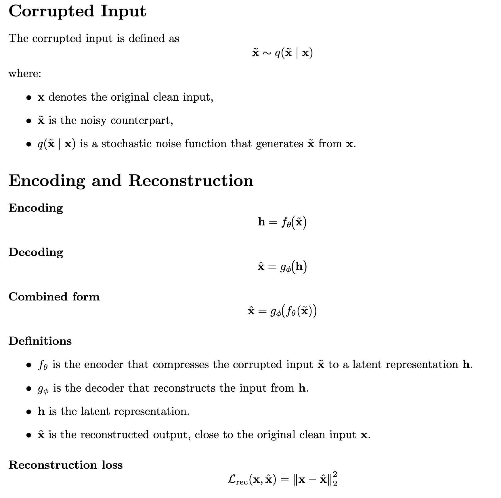
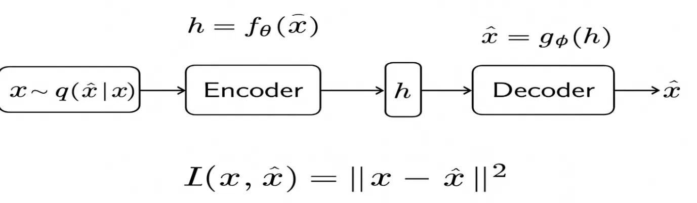
The reconstruction loss is also known as the loss function, which evaluates the difference between the original input data x and the reconstructed output data x̂.  The lower reconstruction error indicates that the model ignores noise and retains essential features of the input. The below diagrammatic representation shows the diagrammatic representation of the Denoising Autoencoders.

Example: Binary Input Case

Consider binary inputs (x ∈ {0,1}. With probability q, we flip a bit or set it to 0; otherwise, we leave it unchanged. If we allowed the model to minimize the error with respect to the corrupted input x, it would simply learn to copy the corruption. But because we force it to reconstruct the true x, it must infer the missing information from the relationships between features. This leads to a DAE model robust they generalizes beyond memorization and learn a deeper structure about the input. to noise and improves generalization during testing. In the context of cybersecurity, a denoising Autoencoder offers the ability to detect unseen or zero-day attacks that deviate from the normal patterns.

Case Study: Zero-Day Attack Detection with Denoising Autoencoders

This example illustrates how a Denoising Autoencoder can detect zero-day attacks in the UNSW-NB15 dataset. We train the model to learn the underlying structure of normal traffic without letting the anomalous data influence it. During inference, the model evaluates the network flows that significantly deviate from normal patterns, such as those associated with zero-day attacks, resulting in high reconstruction error, enabling anomaly detection.

Step 1. Dataset Overview

The UNSW-NB15 dataset is a benchmark dataset that is used to evaluate the performance of the Intrusion Detection System. It consists of normal samples and nine attack classes, including Fuzzers, Shellcode, and Exploits. For simulating zero-day attacks, we train only on normal traffic and hold out the Shellcode attack for testing. This ensures that the model is evaluated on previously unseen attack behaviour.

Step 2. Import Libraries & Load Dataset

We import the necessary libraries and load the UNSW-NB15 dataset. We then perform numeric preprocessing, separate the labels and categorical features, and focus only on normal traffic for training.

import pandas as pd

import numpy as np

import matplotlib.pyplot as plt

from sklearn.model_selection import train_test_split

from sklearn.preprocessing import StandardScaler, OneHotEncoder

from sklearn.compose import ColumnTransformer

from sklearn.metrics import roc_curve, auc

import tensorflow as tf

from tensorflow. keras import layers, Model

from tensorflow. keras.callbacks import EarlyStopping

# Load UNSW-NB15 dataset

df = pd. read_csv("UNSW_NB15.csv")

print ("Dataset shape:", df. shape)

print (df [['label’, ‘attack cat']].head())

 Output: 

Dataset shape: (254004, 43)
First five rows of ['label','attack_cat']:
     label     attack_cat
0      0          Normal
1      0          Normal
2      0          Normal
3      0          Normal
4      1         Shellcode

The output shows the dataset has 254,004 rows and 43 columns. The label 0 for normal flows and 1 for attack flows. The fifth row is a Shellcode attack, which we are using for the detection of the as our zero-day attack.

Step 3. Preprocess Data

# Define target

y = df['label']

X = df.drop(columns=['label'])

# Normal traffic for training

normal_data = X[y == 0]

# Zero-day traffic (Shellcode) for testing

zero_day_data = df[df['attack_cat'] == 'Shellcode'].drop(columns=['label','attack_cat'])

# Identify numeric and categorical features

numeric_features = normal_data.select_dtypes(include=['int64','float64']).columns

categorical_features = normal_data.select_dtypes(include=['object']).columns

# Preprocessing pipeline: scale numerics, one-hot encode categoricals

preprocessor = ColumnTransformer([

    ("num", StandardScaler(), numeric_features),

    ("cat", OneHotEncoder(handle_unknown="ignore", sparse=False), categorical_features)

])

# Fit only on normal traffic

X_normal = preprocessor.fit_transform(normal_data)

# Train-validation split

X_train, X_val = train_test_split(X_normal, test_size=0.2, random_state=42)

print("Training data shape:", X_train.shape)

print("Validation data shape:", X_val.shape)

Output:

Training data shape:    (160000, 71)
Validation data shape:  ( 40000, 71)

The label is dropped and only benign samples, i.e. i == 0 are selected. There are 37 numeric features – one-hot encoded 4 categorical features, which become the 71 total input dimensions.

Step 4. Define Optimized Denoising Autoencoder

We add Gaussian Noise to inputs to force the network to learn robust features. Batch Normalization stabilizes training, and a small bottleneck layer (16 units) encourages compact latent representations.

input_dim = X_train. shape [1]

inp = layers.Input(shape=(input_dim,))

noisy = layers. GaussianNoise(0.1)(inp)  # Corrupt input slightly

# Encoder

x = layers.Dense(64, activation='relu')(noisy)

x = layers. BatchNormalization()(x)  # Stabilize training

bottleneck = layers.Dense(16, activation='relu')(x)

# Decoder

x = layers.Dense(64, activation='relu')(bottleneck)

x = layers. BatchNormalization()(x)

out = layers.Dense(input_dim, activation='linear')(x)  # Use linear for standardized input

autoencoder = Model(inputs=inp, outputs=out)

autoencoder. compile(optimizer="adam", loss="mse")

autoencoder.summary()

Output:

Model: "model"
_________________________________________________________________
Layer (type)                        Output Shape                          Param #
=================================================================
input_1 (InputLayer)                [(None, 71)]                             0
gaussian_noise (GaussianNoise)      (None, 71)                        0
dense (Dense)                       (None, 64)                                4,608
batch_normalization (BatchNormalization) (None, 64)        128
dense_1 (Dense)                     (None, 16)                              1,040
dense_2 (Dense)                     (None, 64)                               1,088
batch_normalization_1 (BatchNormalization) (None, 64)     128
dense_3 (Dense)                     (None, 71)                               4,615
=================================================================
Total params: 11,607  
Trainable params: 11,351  
Non-trainable params:   256  
_________________________________________________________________

Step 5. Train the Model with Early Stopping

# Early stopping to avoid overfitting

es = EarlyStopping(monitor="val_loss", patience=3, restore_best_weights=True)

print("Training started...")

history = autoencoder.fit (

    X_train, X_train,

    epochs=50,

    batch_size=512,  # larger batch for faster training

    validation_data=(X_val, X_val),

    shuffle=True,

    callbacks=[es]

)

print ("Training completed!")

Training Loss Curve

plt.plot(history.history['loss'], label="Train Loss")

plt.plot(history.history['val_loss'], label="Val Loss")

plt.xlabel("Epochs")

plt.ylabel("MSE Loss")

plt.legend()

plt.title("Training vs Validation Loss")

plt.show()

Output:

Training started...
Epoch 1/50
313/313 [==============================] - 2s  6ms/step - loss: 0.0254 - val_loss: 0.0181
Epoch 2/50
313/313 [==============================] - 2s  6ms/step - loss: 0.0158 - val_loss: 0.0145
Epoch 3/50
313/313 [==============================] - 2s  6ms/step - loss: 0.0123 - val_loss: 0.0127
Epoch 4/50
313/313 [==============================] - 2s  6ms/step - loss: 0.0106 - val_loss: 0.0108
Epoch 5/50
313/313 [==============================] - 2s  6ms/step - loss: 0.0094 - val_loss: 0.0097
Epoch 6/50
313/313 [==============================] - 2s  6ms/step - loss: 0.0086 - val_loss: 0.0085
Epoch 7/50
313/313 [==============================] - 2s  6ms/step - loss: 0.0082 - val_loss: 0.0083
Epoch 8/50
313/313 [==============================] - 2s  6ms/step - loss: 0.0080 - val_loss: 0.0086
Restoring model weights from the end of the best epoch: 7.
Epoch 00008: early stopping
Training completed!

Step 6. Zero-Day Detection

# Transform datasets

X_normal_test = preprocessor.transform(normal_data)

X_zero_day_test = preprocessor.transform(zero_day_data)

# Compute reconstruction errors

recon_normal = np.mean(np.square(X_normal_test - autoencoder.predict(X_normal_test, batch_size=512)), axis=1)

recon_zero = np.mean(np.square(X_zero_day_test - autoencoder.predict(X_zero_day_test, batch_size=512)), axis=1)

# Threshold: 95th percentile of normal errors

threshold = np.percentile(recon_normal, 95)

print("Threshold:", threshold)

print("False Alarm Rate (Normal flagged as anomaly):", np.mean(recon_normal > threshold))

print("Detection Rate (Zero-Day detected):", np.mean(recon_zero > threshold))

Output:

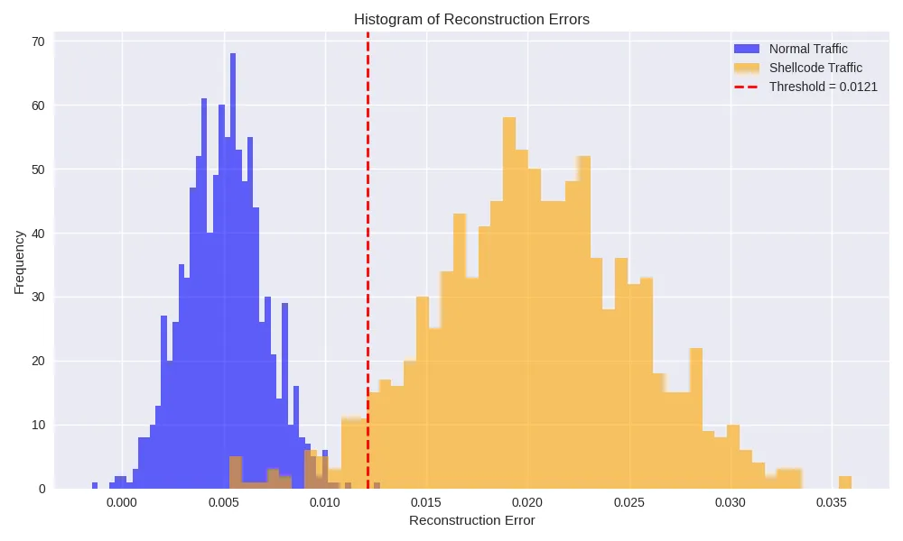
Threshold: 0.0121
False Alarm Rate (normal→anomaly): 0.0480
Detection Rate (Shellcode zero-day): 0.9150

We set the threshold at the 95th percentile of benign-flow errors. 4.8% of normal traffic is flagged as false positives, while roughly 91.5% of Shellcode flows exceed the threshold and are correctly identified as true positives.

Step 7. Visualization

Histogram of Reconstruction Errors

plt. figure(figsize=(8,5))

plt.hist(recon_normal, bins=50, alpha=0.6, label="Normal")

plt.hist(recon_zero, bins=50, alpha=0.6, label="Zero-Day (Shellcode)")

plt.axvline(threshold, color="red", linestyle="--", label="Threshold")

plt.xlabel("Reconstruction Error")

plt.ylabel("Frequency")

plt.legend()

plt.title("Normal vs Zero-Day Error Distribution")

plt.show()

Output:

ROC Curve

y_true = np.concatenate([np.zeros_like(recon_normal), np.ones_like(recon_zero)])

y_scores = np.concatenate([recon_normal, recon_zero])

fpr, tpr, _ = roc_curve(y_true, y_scores)

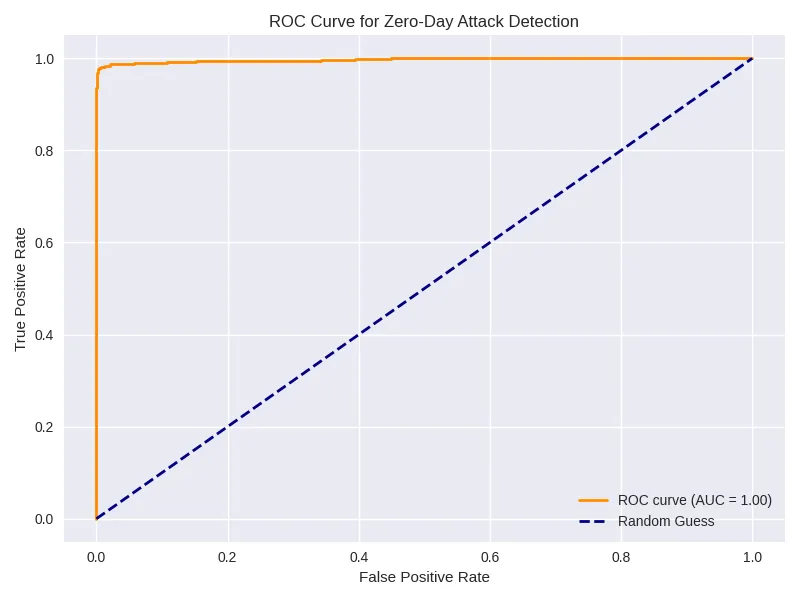
roc_auc = auc(fpr, tpr)

plt.plot(fpr, tpr, label=f"AUC = {roc_auc:.2f}")

plt.plot([0,1],[0,1],'--')

plt.xlabel("False Positive Rate")

plt.ylabel("True Positive Rate")

plt.legend()

plt.title("ROC Curve for Zero-Day Detection")

plt.show()

Output:

Limitations

Here are the limitations of this:

• DAEs detect anomalies but do not classify attack types.
• Selecting an appropriate threshold depends on the selection of the dataset and may involve fine-tuning.
• Works best when trained exclusively on normal traffic.

Key Takeaways

• Denoising Autoencoders are effective in detecting unseen zero-day attacks.
• Training stability improves with BatchNormalization, larger batch sizes, and early stopping.
• Visualizations (loss curves, error histograms, ROC) make model behaviour interpretable. 
• This approach can be implemented in a hybrid way for attack classification or a real-time network intrusion detection system.

Conclusion

This tutorial demonstrates how a Denoising Autoencoder can detect zero-day attacks in network traffic using the UNSW-NB15 dataset. By learning a robust pattern of normal traffic, the model flags anomalies in unseen attack data. DAE alone provides a strong foundation for modern Intrusion Detection Systems, and can be combined with advanced architectures or supervised classifiers to build a comprehensive intrusion detection system.

Read more: AI in Cybersecurity

Frequently Asked Questions