Python Monte Carlo Simulation in Excel

In our data-dominated financial environment, Monte Carlo simulation is a key tool for risk modeling and quantitative strategies. While many of us will continue to use Excel as our preferred platform, it is unfortunate that Excel’s base capabilities require the extra work that many financial professionals will need to complete for any stochastic modeling. In this guide, we will show you how you can ‘plug’ a Monte Carlo simulation in Python into Excel to develop a hybrid optimization for advanced risk analysis and financial modeling. 

Understanding Monte Carlo Simulation in Risk Management

Monte Carlo simulation works by running thousands or millions of random realizations, with the initial input variables defined by probability distributions. The probabilistic modeling approach offers several benefits in situations of uncertain outcomes and financial risk management.

The methodology defines probability distributions for uncertain variables, generates random variates, performs calculations for each realization, and assesses statistical outcomes. Monte Carlo simulation offers insights beyond deterministic models, proving especially useful in portfolio optimization and credit risk modeling.

Risk metrics such as Value-at-Risk (VaR), Expected Shortfall, and probability of loss can be estimated with Monte Carlo estimation. Monte Carlo techniques provide analysts with maximum flexibility to model complex correlations across variables, use non-normal distributions, and account for time-dependent parameters in line with live market conditions.

Python Libraries for Monte Carlo Risk Modeling

Many Python libraries provide outstanding support for Monte Carlo simulation and statistical analysis: 

1. NumPy: NumPy is the backbone due to its powerful array operations and random number generation. It performs vectorized operations, enabling efficient large-scale simulations. The library also provides many statistical functions for probability distributions in financial modeling.
2. SciPy: SciPy builds on NumPy with statistical distributions and optimization algorithms. It offers over 80 distributions and tests for risk modeling. SciPy also supports complex finance applications through numerical integration methods.
3. Pandas: Pandas is highly useful for data manipulation and time series analysis. Its dataframe integrates smoothly with Excel through various import and export functions, making financial data analysis and aggregation straightforward.
4. Matplotlib and Seaborn: Matplotlib and Seaborn enable professional-quality data visualizations of simulation results. These visualizations can include risk distributions or sensitivity analyses, which can be embedded into Excel reports.

Excel Integration Strategies: Python-Excel Connectivity

There are several modern Excel Python integration options, and they have different strengths for Monte Carlo risk modeling:

1. xlwings is the most seamless integration option. This library enables bidirectional communication between Excel and Python, supporting live data exchange and real-time simulation results.
2. openpyxl and xlsxwriter both provide a great file-based integration option to use if a direct connection is not needed. This library enables creating complex reports, handling multiple worksheets, formatting, and charts in Excel from Python simulations. Either library can do the job.
3. COM automation with pywin32 allows for deep integration of Excel on Windows machines, as the library automates the creation and manipulation of Excel objects, ranges, and charts. This option may be beneficial if you want to create sophisticated risk dashboards and interactive modeling environments.

Hands-On Implementation: Building a Monte Carlo Risk Model

It’s time to create a robust portfolio risk analysis system using Excel and a Python Monte Carlo simulation. Using this practical example, we will demonstrate stock price forecasting, correlation analysis, and the computation of risk metrics.

1. Set up the Python environment and prepare the data.

import numpy as np
import pandas as pd
import matplotlib.pyplot as plt
from scipy import stats
from datetime import datetime, timedelta
import warnings
warnings.filterwarnings('ignore')

# Portfolio configuration
stocks = ['AAPL', 'GOOGL', 'MSFT', 'AMZN', 'TSLA']
initial_portfolio_value = 1_000_000
time_horizon = 252
num_simulations = 10000

np.random.seed(42)
annual_returns = np.array([0.15, 0.12, 0.14, 0.18, 0.25])
annual_volatilities = np.array([0.25, 0.22, 0.24, 0.28, 0.35])
portfolio_weights = np.array([0.25, 0.20, 0.25, 0.15, 0.15])

correlation_matrix = np.array([
    [1.00, 0.65, 0.72, 0.58, 0.45],
    [0.65, 1.00, 0.68, 0.62, 0.38],
    [0.72, 0.68, 1.00, 0.55, 0.42],
    [0.58, 0.62, 0.55, 1.00, 0.48],
    [0.45, 0.38, 0.42, 0.48, 1.00]
])

2. Monte Carlo Simulation Engine

def monte_carlo_portfolio_simulation(returns, volatilities, correlation_matrix,
                                     weights, initial_value, time_horizon, num_sims):
    # Convert annual parameters to daily
    daily_returns = returns / 252
    daily_volatilities = volatilities / np.sqrt(252)

    # Generate correlated random returns
    L = np.linalg.cholesky(correlation_matrix)

    # Storage for simulation results
    portfolio_values = np.zeros((num_sims, time_horizon + 1))
    portfolio_values[:, 0] = initial_value

    # Run Monte Carlo simulation
    for sim in range(num_sims):
        random_shocks = np.random.normal(0, 1, (time_horizon, len(stocks)))
        correlated_shocks = random_shocks @ L.T

        daily_asset_returns = daily_returns + daily_volatilities * correlated_shocks
        portfolio_daily_returns = np.sum(daily_asset_returns * weights, axis=1)

        for day in range(time_horizon):
            portfolio_values[sim, day + 1] = portfolio_values[sim, day] * (1 + portfolio_daily_returns[day])

    return portfolio_values

# Execute simulation
print("Running Monte Carlo simulation...")
simulation_results = monte_carlo_portfolio_simulation(
    annual_returns, annual_volatilities, correlation_matrix,
    portfolio_weights, initial_portfolio_value, time_horizon, num_simulations
)

3. Risk Metrics Calculation and Analysis

def calculate_risk_metrics(portfolio_values, confidence_levels=[0.95, 0.99]):
    final_values = portfolio_values[:, -1]
    returns = (final_values - portfolio_values[:, 0]) / portfolio_values[:, 0]
    losses = -returns

    mean_return = np.mean(returns)
    volatility = np.std(returns)

    # VaR
    var_metrics = {}
    for confidence in confidence_levels:
        var_metrics[f'VaR_{int(confidence*100)}%'] = np.percentile(losses, confidence * 100)

    # Expected Shortfall
    es_metrics = {}
    for confidence in confidence_levels:
        threshold = np.percentile(losses, confidence * 100)
        es_metrics[f'ES_{int(confidence*100)}%'] = np.mean(losses[losses >= threshold])

    max_loss = np.max(losses)
    prob_loss = np.mean(returns < 0)
    sharpe_ratio = mean_return / volatility if volatility > 0 else 0

    return {
        'mean_return': mean_return,
        'volatility': volatility,
        'sharpe_ratio': sharpe_ratio,
        'max_loss': max_loss,
        'prob_loss': prob_loss,
        **var_metrics,
        **es_metrics
    }

risk_metrics = calculate_risk_metrics(simulation_results)

4. Excel Integration and Dashboard Creation

def create_excel_risk_dashboard(simulation_results, risk_metrics, stocks, weights):
    portfolio_data = pd.DataFrame({
        "Stock": stocks,
        "Weight": weights,
        "Expected Return": annual_returns,
        "Volatility": annual_volatilities
    })

    metrics_df = pd.DataFrame(list(risk_metrics.items()), columns=['Metric', 'Value'])
    metrics_df['Value'] = metrics_df['Value'].round(4)

    final_values = simulation_results[:, -1]
    # Excel export code would follow here

summary_stats = {
    "Initial Portfolio Value": f"${initial_portfolio_value:,.0f}",
    "Mean Final Value": f"${np.mean(final_values):,.0f}",
    "Median Final Value": f"${np.median(final_values):,.0f}",
    "Standard Deviation": f"${np.std(final_values):,.0f}",
    "Minimum Value": f"${np.min(final_values):,.0f}",
    "Maximum Value": f"${np.max(final_values):,.0f}"
}

summary_df = pd.DataFrame(list(summary_stats.items()), columns=['Statistic', 'Value'])

plt.figure(figsize=(10, 6))
plt.hist(final_values, bins=50, alpha=0.7, color="skyblue", edgecolor="black")

plt.axvline(initial_portfolio_value, color="red", linestyle="--",
            label=f'Initial Value: ${initial_portfolio_value:,.0f}')
plt.axvline(np.mean(final_values), color="green", linestyle="--",
            label=f'Mean Final Value: ${np.mean(final_values):,.0f}')

var_95 = initial_portfolio_value * (1 - risk_metrics['VaR_95%'])
plt.axvline(var_95, color="orange", linestyle="--",
            label=f'95% VaR: ${var_95:,.0f}')

plt.title("Portfolio Value Distribution - Monte Carlo Simulation")
plt.xlabel("Portfolio Value ($)")
plt.ylabel("Frequency")
plt.legend()
plt.grid(True, alpha=0.3)
plt.savefig("portfolio_distribution.png", dpi=300, bbox_inches="tight")
plt.close()

5. Advanced Scenario Analysis

def scenario_stress_testing(base_returns, base_volatilities,             correlation_matrix, weights, initial_value, scenarios):
    scenario_results = {}
    for scenario_name, (return_shock, vol_shock) in scenarios.items():
        stressed_returns = base_returns + return_shock
        stressed_volatilities = base_volatilities * (1 + vol_shock)

        scenario_sim = monte_carlo_portfolio_simulation(
            stressed_returns, stressed_volatilities, correlation_matrix,
            weights, initial_value, time_horizon, 5000
        )

        scenario_metrics = calculate_risk_metrics(scenario_sim)
        scenario_results[scenario_name] = scenario_metrics

    return scenario_results


stress_scenarios = {
    "Base Case": (0.0, 0.0),
    "Market Crash": (-0.20, 0.5),
    "Bear Market": (-0.10, 0.3),
    "High Volatility": (0.0, 0.8),
    "Recession": (-0.15, 0.4)
}

scenario_results = scenario_stress_testing(
    annual_returns, annual_volatilities, correlation_matrix,
    portfolio_weights, initial_portfolio_value, stress_scenarios
)

scenario_df = pd.DataFrame(scenario_results).T.round(4)

OUTPUT:

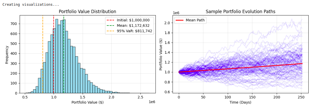
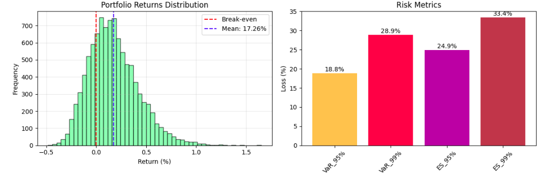
Output Analysis:

The Monte Carlo-type simulation outputs provide a comprehensive understanding of risk analysis through key statistics and visualizations of potential portfolio behavior in uncertainty. The Value-at-Risk (VaR) methodologies typically indicate for a diversified portfolio a 5% chance of experiencing more than a 15-20% drop in value over a 1-year time horizon. The Expected Shortfall metrics state the average losses of bad outcomes. The histogram of the portfolio value distribution gives the probabilistic range of outcomes, often demonstrating a right skewness pattern with respect to risk on the downside being concentrated, while the upside potential remains. 

Risk-adjusted performance statistics, such as the Sharpe ratio (usually measured in the range of 0.8 to 1.5 for portfolios with balanced exposure), can indicate if the potential expected return justifies the volatility exposure. The visualization of simulation paths indicates that market uncertainty is compounded over time, with individual scenarios diverging far away from the mean trajectory, and the directional changes that occur over time provide potential insight into strategic asset allocation or risk management decisions.

Advanced Techniques: Enhancing Monte Carlo Risk Models

By utilizing variance reduction techniques, efficiency and accuracy in Monte Carlo simulations can be substantially improved. 

• Antithetic variates, control variates, and importance sampling methods reduce the required number of simulations to reach the level of precision that is desired.
• Quasi-Monte Carlo methods are based upon low-discrepancy sequences such as `Sobol` or `Halton repeats, which will often converge faster than pseudo-random methods, especially for high-dimensional derivative pricing and portfolio optimization problems. 
• Copula-based dependency modeling capabilities use more sophisticated correlation structures than simple linear correlation. `Clayton`, `Gumbel`, and `t-copulas` all can fit tail dependencies and asymmetries among assets to provide realistic estimates of `risk`. 
• Jump diffusion processes and regime-switching models to account for sudden shocks to the market and changing volatility regimes are something pure geometric Brownian motion cannot model. The extended methods will contribute significantly to enhancing stress testing and tail risk analysis.

Read more: A Guide to Monte Carlo Simulation

Conclusion

Using Python Monte Carlo simulation alongside Excel represents a major advance in quantitative risk management. This hybridized version effectively uses the computational rigor of Python coupled with the usability of Excel, resulting in advanced risk modeling tools that retain usability enhancement along with functionality. This means financial professionals can perform advanced scenario analysis, stress testing, and portfolio optimization while capitalizing on the familiarity of the Excel platform. The methodologies included in this tutorial provide a paradigm on how to construct enterprise-wide risk management systems, where both analytical rigor and usability can meet the same destination. 

In an ever-evolving regulatory and complex market environment, the enhanced capacity for adaptation and advancement of risk models will become ever more relevant. Integrating Python-Excel allows us to achieve the flexibility and technical capabilities to shoulder these challenges while enhancing the transparency and auditability of risk management model development. 

Frequently Asked Questions